Two-node examples
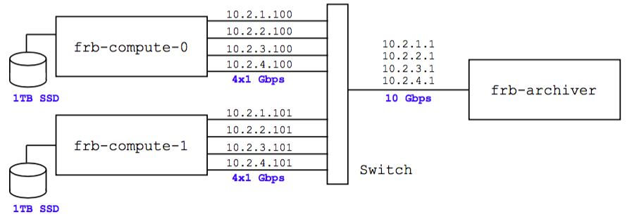
For now, the “two-node McGill backend” refers to the network below. The nodes are in a non-link-bonded configuration, with each of their four 1 Gbps NIC’s on a separate /24 network. (Note: this figure is out of date, since the frb-archiver no longer exists, but I was too lazy to make a new figure.)
Example 3
This is a 16-beam production-scale example. It uses “placeholder” RFI removal (which detrends the data but doesn’t actually remove RFI), and the least optimal bonsai configuaration (no low-DM upsampled tree or spectral index search). As remarked above, this is currently the best we can do with 16 beams/node, due to the RFI removal running slower than originally hoped!
This is a two-node example, with the L0 simulator running on frb-compute-0, and the L1 server running on frb-compute-1. We process 16 beams with 16384 frequency channels and 1 ms sampling. The total bandwidth is 2.2 Gbps, distributed on 4x1 Gbps NIC’s by assigning four beams to each NIC.
Because of the “slow start” problem described previously in Caveats, this example is now a 20-minute run (previously, it was a 5-minute run).
On
frb-compute-1, start the L1 server:./ch-frb-l1 \ l1_configs/l1_example3.yaml \ rfi_configs/rfi_placeholder.json \ /data/bonsai_configs/bonsai_production_noups_nbeta1_v2.hdf5 \ l1b_config_placeholderIt may take around 30 seconds for all threads and processes to start! Before going on to the next step, you should wait until messages of the form “toy-l1b.py: starting…” appear.
Note: On frb-compute-1 and the other CHIME nodes, the bonsai “production” HDF5 files have been precomputed for convenience, and are kept in /data/bonsai_configs. This is why we were able to skip the step of computing the .hdf5 file from bonsai_configs/bonsai_production_noups_nbeta1_v2.txt.
On
frb-compute-0, start the L0 simulator:./ch-frb-simulate-l0 l0_configs/l0_example3.yaml 1200This simulates 20 minutes of data. If you switch back to the L1 server window, you’ll see some incremental output every 10 seconds or so, as coarse-grained triggers are received by the toy-l1b processes.
When the simulation ends (after 20 minutes), the toy-l1b processes will write their trigger plots (toy_l1b_beam*.png). These will be large files (20000-by-4000 pixels)!
Notes on the two-node backend:
Right now the following ports are open on the firewalls of the compute nodes: 5555/tcp, 6677/udp, 6677/tcp. If you need to open more, the syntax is:
sudo firewall-cmd --zone=public --add-port=10252/udp --permanent
sudo firewall-cmd --reload
sudo firewall-cmd --list-all
You may run into a nuisance issue where the L1 process hangs for a long time (uninterruptible with control-C) after throwing an exception, because it is trying to write its core dump. My solution is
sudo killall -9 abrt-hook-ccppin another window. Let me know if you find a better one!A related issue: core dumps can easily fill the / filesystem. My solution here is:
sudo su
rm -rf /var/spool/abrt/ccpp*
exit
…but be careful with rm -rf as root!
Example 4
This is an 8-beam production-scale example. It uses a real RFI removal scheme developed by Masoud (but out-of-date compared to what we’re currently using in the real-time search), and the most optimal bonsai configuration (with a low-DM upsampled tree and two trial spectral indices).
On
frb-compute-1, start the L1 server:./ch-frb-l1 \ l1_configs/l1_example4.yaml \ rfi_configs/rfi_production_v1.json \ /data/bonsai_configs/bonsai_production_ups_nbeta2_v2.hdf5 \ l1b_config_placeholderand wait for it to finish initializing (takes around 1 minute).
On
frb-compute-0, start the L0 simulator:./ch-frb-simulate-l0 l0_configs/l0_example4.yaml 1200